Pivot tables in Excel are a powerful data analysis tool that allows you to summarize, manipulate, and analyze large amounts of data efficiently. They can help you gain insights, make data-driven decisions, and present information in a visual and organized manner. In this blog, we will walk you through the steps of creating and working with a pivot table in Excel. 

Step 1: Preparing Your Data 

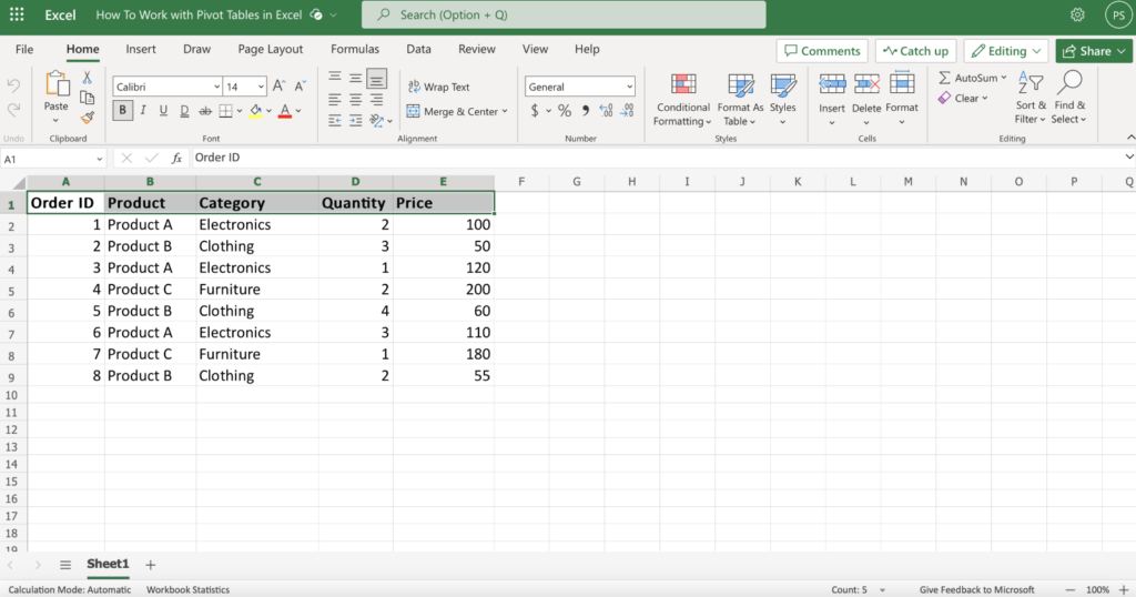
Before creating a pivot table, it is essential to ensure that your data is organized in a tabular format. Each column should have a unique heading, and there should be no blank rows or columns within the dataset. Here are the steps to prepare your data: 

1. Open Excel and navigate to the worksheet containing your data. 

2. Ensure that the headers for each column are meaningful and descriptive. 

3. Remove any unnecessary or irrelevant columns that may clutter your analysis. 

4. Check for and remove any empty rows or columns. 

5. Save your changes. 

Step 2: Selecting Your Data Range 

The next step is to select the range of data on which you want to create the pivot table. Follow these steps to select your data range: 

6. Click on any cell within your dataset. 

7. Press Ctrl + Shift + Right Arrow to select the entire row. 

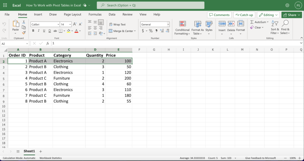
8. Press Ctrl + Shift + Down Arrow to select all the rows in the column. 

9. Repeat steps 2 and 3 for each additional column you want to include. 

Step 3: Inserting a Pivot Table 

Once you have selected your data range, it’s time to create a pivot table. Here’s how you can insert a pivot table: 

10. Go to the “Insert” tab on the Excel ribbon. 

11. Click on the “PivotTable” button. A dialogue box will appear. 

12. Ensure that the “Select a table or range” option is selected. 

13. Verify that the correct data range is shown in the “Table/Range” field. 

14. Choose whether you want the pivot table to be placed on a new worksheet or an existing worksheet. 

15. Click “OK.” 

Step 4: Configuring the Pivot Table 

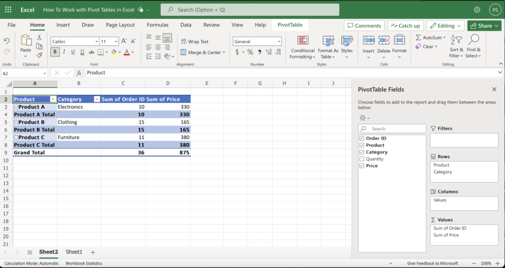
After inserting a pivot table, you will need to configure it based on your specific requirements. Here are some essential steps to follow: 

16. Drag and drop the relevant fields from the “PivotTable Field List” onto the “Rows,” “Columns,” or “Values” section. 

17. To summarize the data, choose an appropriate summary function (e.g., sum, count, average) for the value fields. 

18. To filter the data, drag a field to the “Report Filter” section. This allows you to focus on specific subsets of your data. 

19. Rearrange the fields within the pivot table by dragging them to different positions for better understanding and analysis. 

20. Customize the format, style, and design of your pivot table using various options available in the “Design” and “Analyze” tabs. 

Step 5: Updating and Refreshing the Pivot Table 

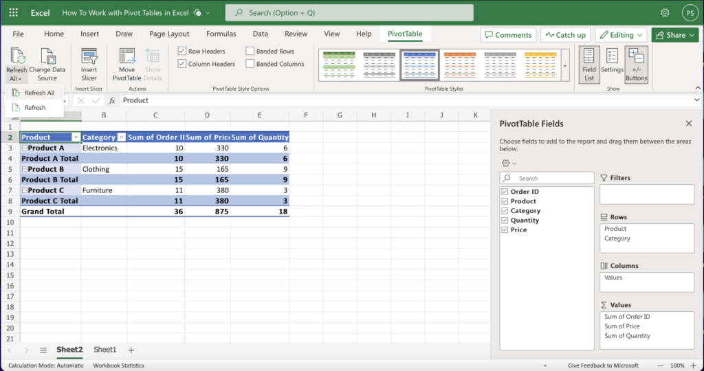
As you make changes to your source data, you will need to update and refresh the pivot table to reflect those changes. Follow these steps to update your pivot table: 

21. Right-click anywhere within the pivot table. 

22. Click on “Refresh” or “Refresh All” to update the entire workbook if you have multiple pivot tables. 

23. Alternatively, you can use the “Refresh” button from the “Data” tab to update the pivot table. 

Conclusion 

Pivot tables in Excel are an invaluable tool for data analysis and provide a simple and effective way to summarize and analyze large datasets. By following the steps outlined above, you can create pivot tables, and manipulate and customize them to derive meaningful insights from your data. Experiment with different configurations and features to explore the full potential of pivot tables in Excel.